Geromont and Butterworth (2015) Constant Catch
CC1.RdThe TAC is the average historical catch over the last yrsmth (default 5) years,
multiplied by (1-xx)
CC1(x, Data, reps = 100, plot = FALSE, yrsmth = 5, xx = 0)

CC2(x, Data, reps = 100, plot = FALSE, yrsmth = 5, xx = 0.1)

CC3(x, Data, reps = 100, plot = FALSE, yrsmth = 5, xx = 0.2)

CC4(x, Data, reps = 100, plot = FALSE, yrsmth = 5, xx = 0.3)

CC5(x, Data, reps = 100, plot = FALSE, yrsmth = 5, xx = 0.4)

CurC(x, Data, reps = 100, plot = FALSE, yrsmth = 1, xx = 0)
Arguments
| x | A position in the data object |
|---|---|
| Data | A data object |
| reps | The number of stochastic samples of the MP recommendation(s) |
| plot | Logical. Show the plot? |
| yrsmth | Years over which to calculate mean catches |
| xx | Parameter controlling the TAC. Mean catches are multiplied by
(1- |
Value
An object of class Rec with the TAC slot populated with a numeric vector of length reps
Details
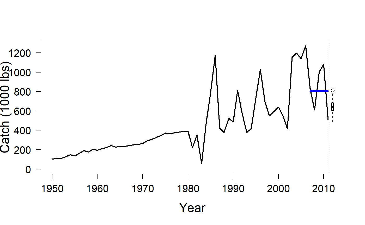
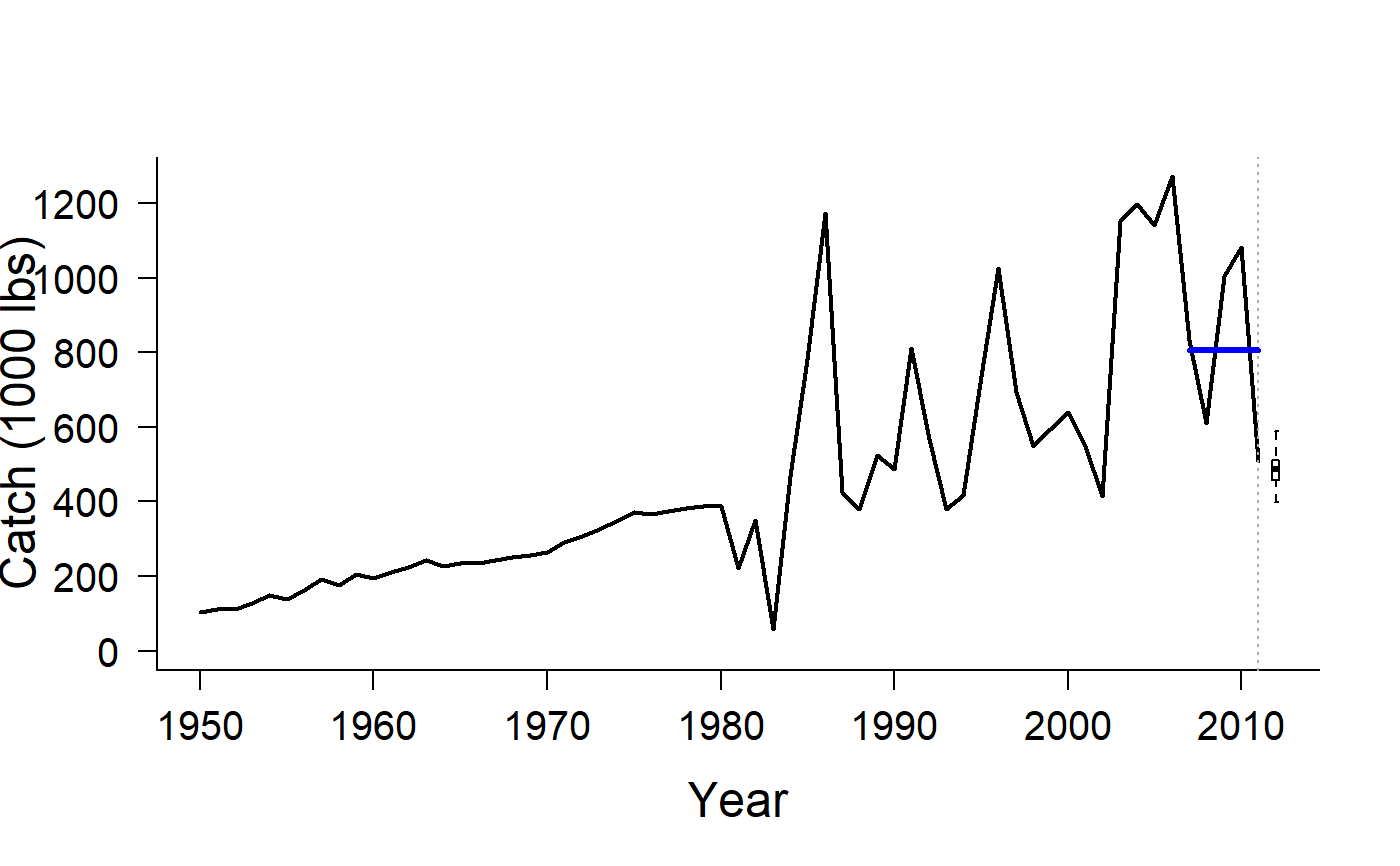
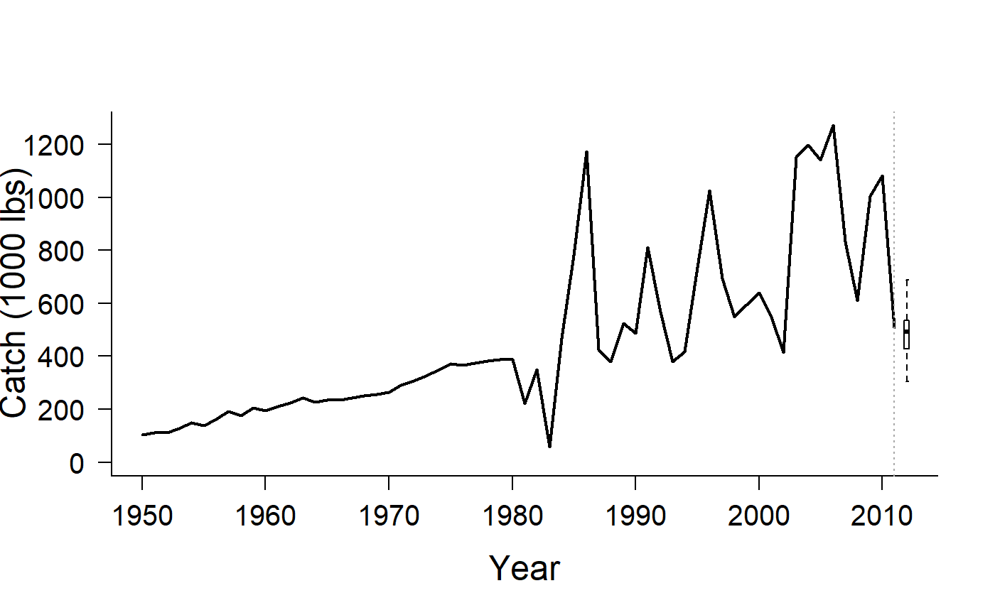
The TAC is calculated as:
$$\textrm{TAC} = (1-x)C_{\textrm{ave}}$$
where x lies between 0 and 1, and \(C_{\textrm{ave}}\) is average historical
catch over the previous yrsmth years.
The TAC is constant for all future projections.
Functions
CC1: TAC is average historical catch from recentyrsmthyearsCC2: TAC is average historical catch from recentyrsmthyears reduced by 10\CC3: TAC is average historical catch from recentyrsmthyears reduced by 20\CC4: TAC is average historical catch from recentyrsmthyears reduced by 30\CC5: TAC is average historical catch from recentyrsmthyears reduced by 40\CurC: TAC is fixed at last historical catch
Required Data
See Data for information on the Data object
CC1: Cat, LHYear, Year
Rendered Equations
See Online Documentation for correctly rendered equations
References
Geromont, H. F., and D. S. Butterworth. 2015. Generic Management Procedures for Data-Poor Fisheries: Forecasting with Few Data. ICES Journal of Marine Science: Journal Du Conseil 72 (1). 251-61.
See also
Other Constant Catch MPs:
GB_CC()
Examples
#> TAC (median) #> 793.0111#> TAC (median) #> 721.9369#> TAC (median) #> 640.544#> TAC (median) #> 548.6459#> TAC (median) #> 485.7275#> TAC (median) #> 491.539