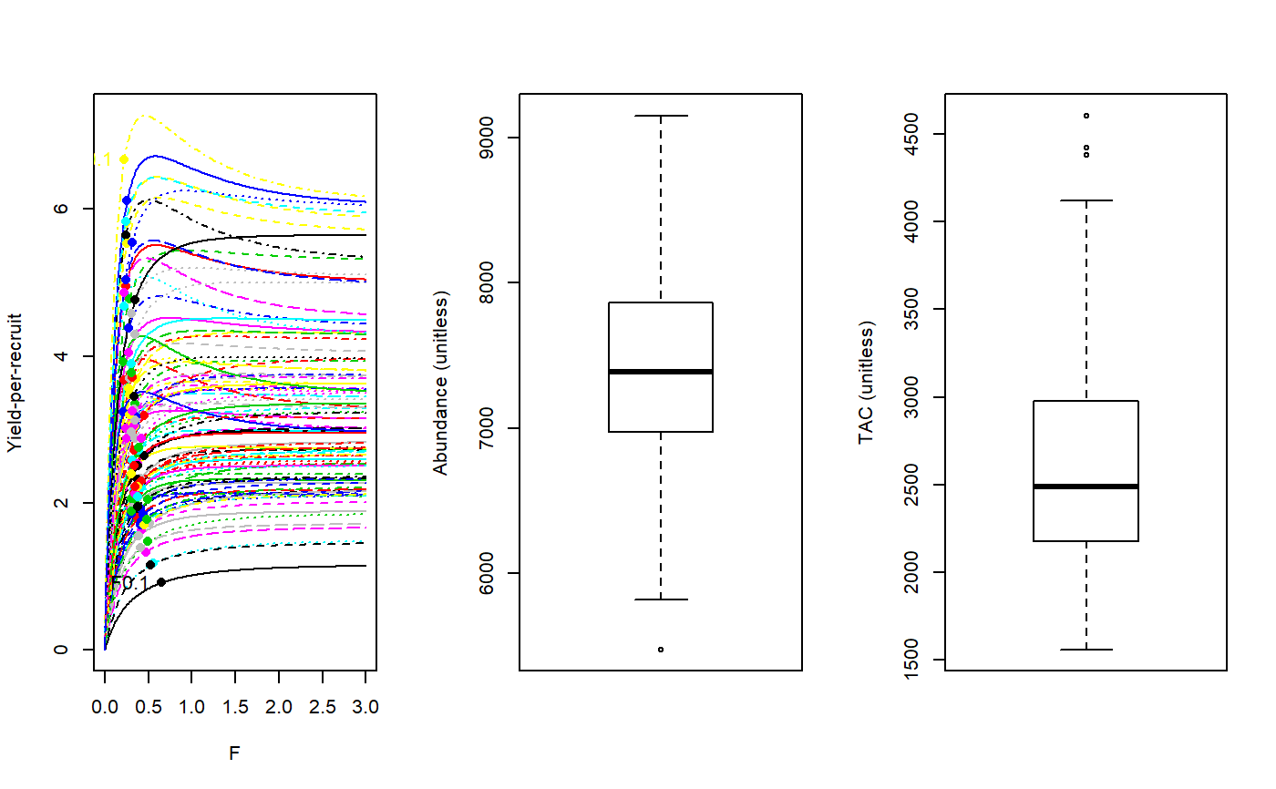
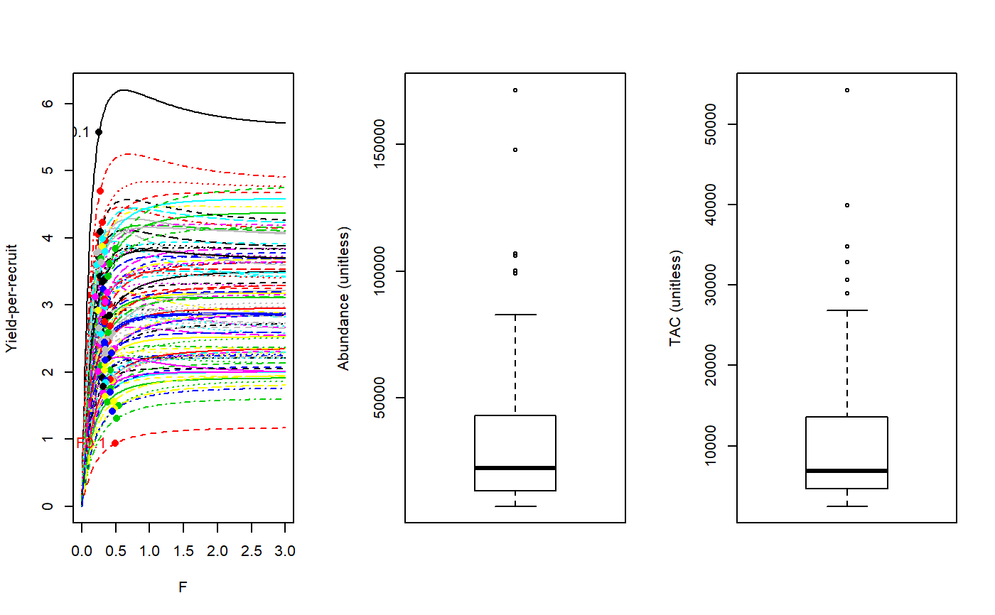
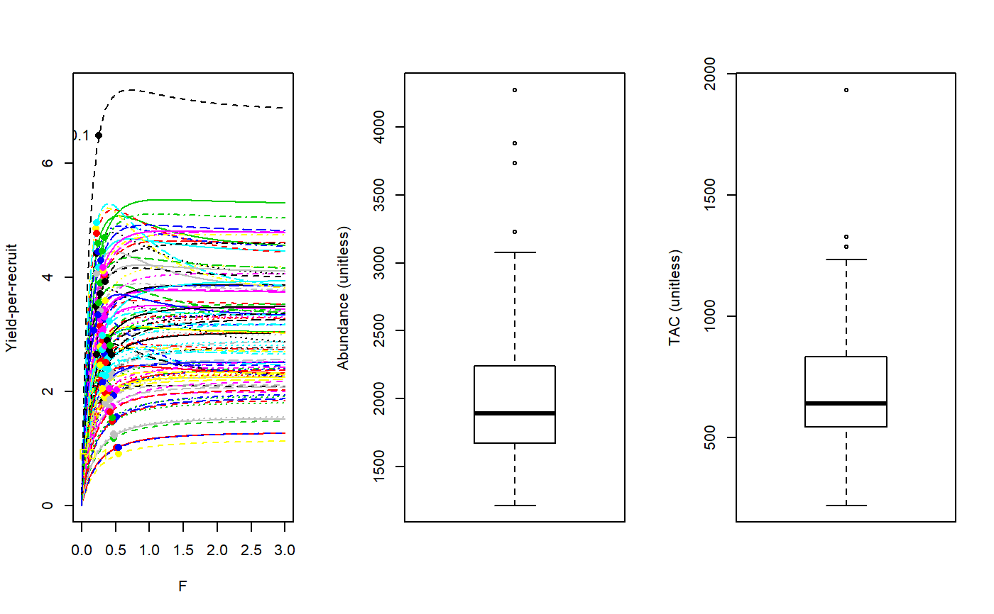
Yield Per Recruit analysis to get FMSY proxy F01
YPR.RdA simple yield per recruit approximation to FMSY (F01) which is the position of the ascending YPR curve for which dYPR/dF = 0.1(dYPR/d0)
YPR(x, Data, reps = 100, plot = FALSE)

YPR_CC(x, Data, reps = 100, plot = FALSE, Fmin = 0.005)

YPR_ML(x, Data, reps = 100, plot = FALSE)
Arguments
| x | A position in the data object |
|---|---|
| Data | A data object |
| reps | The number of stochastic samples of the MP recommendation(s) |
| plot | Logical. Show the plot? |
| Fmin | The minimum fishing mortality rate inferred from the catch-curve analysis |
Value
An object of class Rec with the TAC slot populated with a numeric vector of length reps
Details
The TAC is calculated as: $$\textrm{TAC} = F_{0.1} A$$ where \(F_{0.1}\) is the fishing mortality (F) where the slope of the yield-per-recruit (YPR) curve is 10\
The YPR curve is calculated using an equilibrium age-structured model with life-history and
selectivity parameters sampled from the Data object.
The variants of the YPR MP differ in the method to estimate current abundance (see Functions section below). #'
Functions
YPR: Requires an external estimate of abundance.YPR_CC: A catch-curve analysis is used to determine recent Z which given M (Mort) gives F and thus abundance = Ct/(1-exp(-F))YPR_ML: A mean-length estimate of recent Z is used to infer current abundance.
Note
Based on the code of Meaghan Bryan
Required Data
See Data for information on the Data object
YPR: Abun, LFS, MaxAge, vbK, vbLinf, vbt0
YPR_CC: CAA, Cat, LFS, MaxAge, vbK, vbLinf, vbt0
YPR_ML: CAL, Cat, Lbar, Lc, LFS, MaxAge, Mort, vbK, vbLinf, vbt0
Rendered Equations
See Online Documentation for correctly rendered equations
References
Beverton and Holt. 1954.
Examples
#> TAC (median) #> 2486.766#> TAC (median) #> 6908.574#> TAC (median) #> 639.3885