Chapter 3 A Very Quick Demo

Running an MSE with DLMtool is quite straightforward and only requires a single line of code:

myMSE <- runMSE()

If you run this line (remember, if you haven’t already you must first run library(DLMtool)) and see something similiar to the output shown here, then DLMtool is successfully working on your system.

If the MSE did not run successfully, repeat the previous steps, ensuring that you have the latest version of R and the DLMtool package. If still no success, please contact us with a description of the problem and we will try to help.

Once an MSE is run, the results can be examined visually using plotting functions, for example:

Pplot(myMSE)

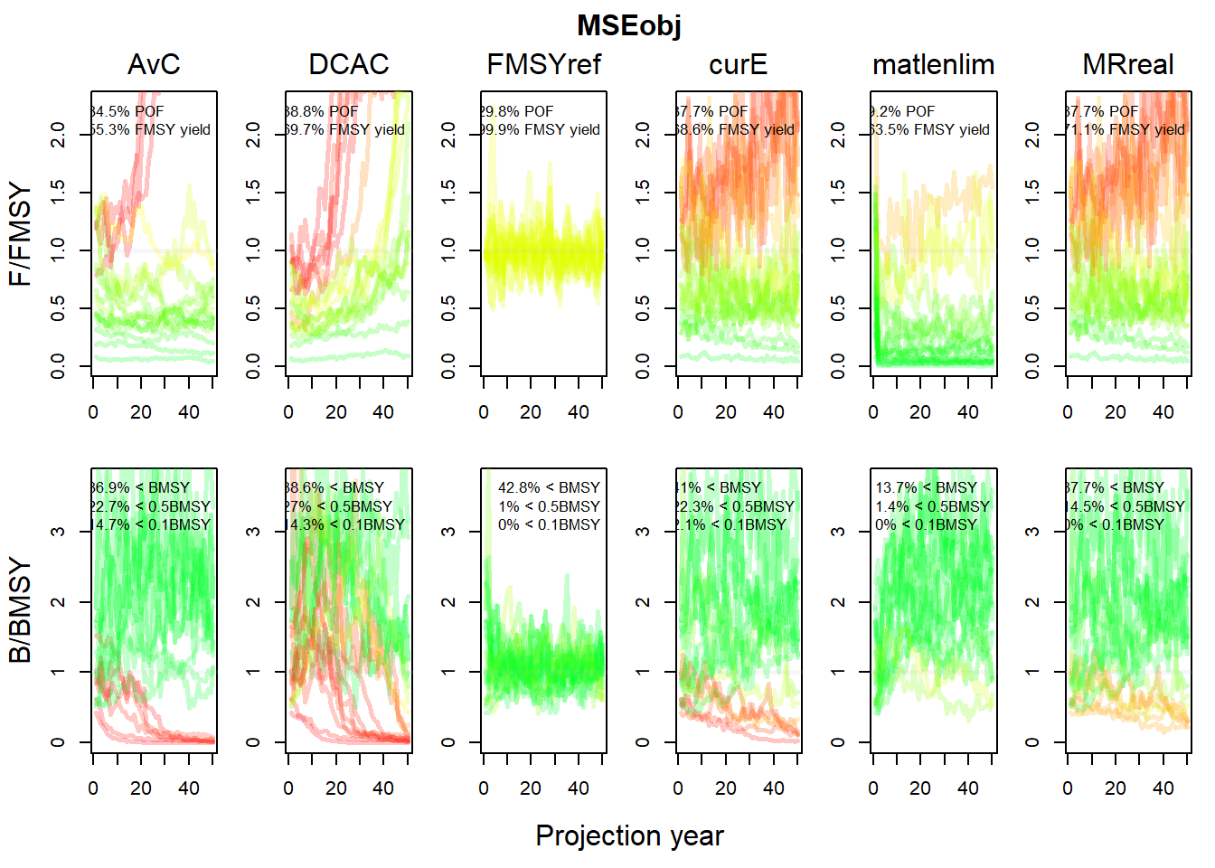
Or quantified in various ways, for example:

summary(myMSE)

## Calculating Performance Metrics

##                                       Performance.Metrics                                            
## 1                 Probability of not overfishing (F<FMSY)               Prob. F < FMSY (Years 1 - 50)
## 2                      Spawning Biomass relative to SBMSY         Prob. SB > 0.5 SBMSY (Years 1 - 50)
## 3        Average Annual Variability in Yield (Years 1-50)               Prob. AAVY < 20% (Years 1-50)
## 4 Average Yield relative to Reference Yield (Years 41-50)  Prob. Yield > 0.5 Ref. Yield (Years 41-50)
## 
## 
## Performance Statistics:
##          MP PNOF  P50 AAVY  LTY
## 1       AvC 0.71 0.80 1.00 0.62
## 2      DCAC 0.64 0.76 1.00 0.65
## 3   FMSYref 0.68 0.99 1.00 1.00
## 4      curE 0.71 0.87 0.21 0.79
## 5 matlenlim 0.96 0.99 0.23 0.60
## 6    MRreal 0.71 0.92 0.23 0.80

Later sections of the user manual will describe more ways to evaluate the outputs of the runMSE function. But first we will look at the most fundamental part of MSE: the Operating Model.