Chapter 14 Examining the MSE object
The MSE object contains all of the output from the MSE. In this chapter we will examine the MSE object in more detail.
First we will run an MSE so that we have an MSE object to work with. We will then briefly examine some of the contents of the MSE object. The chapters Performance Metrics and Custom Performance Metrics contain more information on the MSE object.
We create an OM based on the Blue Shark stock object and other built-in objects:
Note that we have increased the number of simulations from the default 48 to 200:
## [1] 200Let’s choose an arbitrary set of MPs:
Set up parallel processing:
## Library DLMtool loaded.And run the MSE using parallel processing and save the output to an object called BSharkMSE:
## Running MSE in parallel on 10 processors## MSE completedThe names of the slots in an object of class MSE can be displayed using the slotNames function:
##  [1] "Name"     "nyears"   "proyears" "nMPs"     "MPs"      "nsim"     "OM"       "Obs"      "B_BMSY"   "F_FMSY"
## [11] "B"        "SSB"      "VB"       "FM"       "C"        "TAC"      "SSB_hist" "CB_hist"  "FM_hist"  "Effort"
## [21] "PAA"      "CAA"      "CAL"      "CALbins"  "Misc"
As you can see, MSE objects contain all of the information from the MSE, stored in 25 slots.
14.1 The First Six Slots
The first six slots contain information on the structure of the MSE. For example the first slot (Name), is a combination of the names of the Stock, Fleet, and Obs objects that were used in the MSE:
## [1] "Stock:Blue shark Fleet:Generic_Fleet Obs model:Imprecise-Biased Imp model:Perfect_Imp"Other information in these first slots includes the number of historical years (nyears), the number of projection years (proyears), the number of name of the Management Procedures (nMPs and MPs), and the number of simulations (nsim).
14.2 The OM Slot
The OM slot in the MSE object is a data frame that the values of the parameters used in the Operating Model:
##  [1] "A"            "AC"           "ageM"         "Asp"          "Blow"         "BMSY"         "BMSY_B0"
##  [8] "CurrentYr"    "D"            "dFfinal"      "DR"           "Esd"          "Fdisc"        "FinF"
## [15] "FMSY"         "FMSY_M"       "Frac_area_1"  "hs"           "K"            "Ksd"          "L5"
## [22] "L50"          "L50_95"       "L95"          "LenCV"        "LFR"          "LFS"          "Linf"
## [29] "Linfsd"       "LR5"          "M"            "maxF"         "maxlen"       "Mexp"         "MGT"
## [36] "Msd"          "MSY"          "OFLreal"      "Prob_staying" "procmu"       "procsd"       "qcv"
## [43] "qinc"         "R0"           "RefY"         "Rmaxlen"      "Size_area_1"  "SizeLimFrac"  "SizeLimSD"
## [50] "Spat_targ"    "SRrel"        "SSB0"         "SSBMSY"       "SSBMSY_SSB0"  "t0"           "TACFrac"
## [57] "TACSD"        "TAEFrac"      "TAESD"        "UMSY"         "Vmaxlen"
If you use the dim function to report the dimensions of the OM data frame, you’ll notice that there are 61 columns, corresponding to the 61 parameters in the Operating Model, and 200 rows, each corresponding to a single simulation of the MSE.
More information on the MSE@OM slot can be found in the help documentation: class?MSE
14.3 The Obs Slot
The Obs slot contains another data frame, this one with 26 columns corresponding to the values drawn from the Observation model:
##  [1] "Abias"       "Aerr"        "betas"       "BMSY_B0bias" "Brefbias"    "CAA_ESS"     "CAA_nsamp"   "CAL_ESS"
##  [9] "CAL_nsamp"   "Cbias"       "Crefbias"    "Csd"         "Dbias"       "Derr"        "FMSY_Mbias"  "hbias"
## [17] "Irefbias"    "Isd"         "Kbias"       "lenMbias"    "LFCbias"     "LFSbias"     "Linfbias"    "Mbias"
## [25] "Recsd"       "t0bias"
The Obs data frame also has 200 rows, each corresponding to a single simulation. More information on the MSE@Obs slot can be found in the help documentation: class?MSE
The information contained in the OM and Obs slots can be used to examine the sensitivity of the performance of Management Procedures with respect to different operating model and observation parameters. This is discussed in more detail below.
14.4 The B_BMSY and F_FMSY Slots
The B_BMSY and F_FMSY are data frames containing the biomass relative to biomass at maximum sustainable yield \(\left(\frac{B}{B_{MSY}}\right)\), and fishing mortality relative to the rate corresponding to maximum sustainable yield \(\left(\frac{F}{F_{MSY}}\right)\) for each simulation, Management Procedure and projection year.
If we look at the class of the B_BMSY slot, we see that it is an array:
## [1] "array"Using the dim function we can see that it is a 3-dimensional array, with the size corresponding to the number of simulations (nsim), the number of Management Procedures (nMPs), and the number of projection years (proyears):
## [1] 200 5 50This information can be used to calculate statistics relating to the performance of each Management Procedure with respect to these metrics.
For example, if you wish to look at the distribution of \(\frac{B}{B_{MSY}}\) for the second Management Procedure (DCAC), you could use the boxplot function:
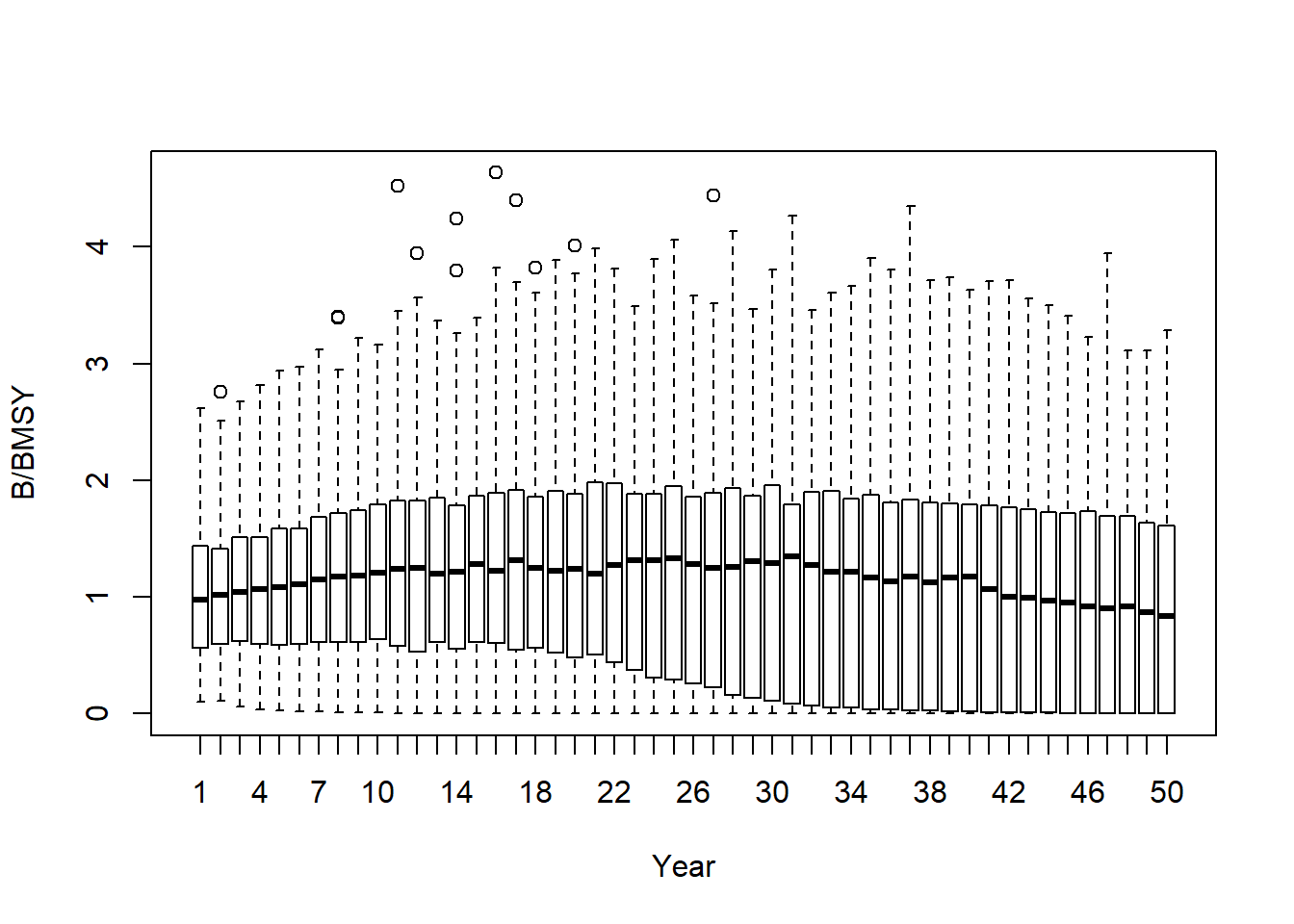
This plot shows that the relative biomass for the stock generally increases through the projection period when the DCAC method is used, with the median relative biomass increasing from about 0.98 in the first year to 0.83 in the final year.
However, the distribution appears to have quite high variability, which suggests that although the method works well on average, the final biomass was very low in some simulations.
14.5 The B, FM, C and TAC Slots
The B, FM, and C slots contain the information relating to the stock biomass, the fishing mortality rate, and the catch for each simulation, Management Procedure, and projection year.
Typically, the MSE model in the DLMtool does not include information on the absolute scale of the stock biomass or recruitment, and all results usually must be interpreted in a relativistic context.
This is particularly true for the biomass (B) and catch (C) where the absolute values in the MSE results (other than 0!) have little meaning.
The biomass can by made relative to \(B_{MSY}\), as shown above. Alternatively, biomass can be calculated with respect to the unfished biomass \(\left(B_0\right)\), from information stored in the OM slot.
The catch information is usually made relative to the highest long-term yield (mean over last five years of projection) for each simulation obtained from a fixed F strategy. This information (RefY) can be found in the OM slot.
Alternatively, the catch can be made relative to the catch in last historical year (CB_hist; see below), to see how future catches are expected to change relative to the current conditions.
The TAC slot contains the TAC recommendation for each simulation, MP, and projection year. In cases where a TAC was not set (e.g for a size limit), the value will be NA. The values in TAC may be different to those in the catch (C) slot due to implementation error of the total catch limit.
14.6 The SSB_hist, CB_hist, and FM_hist Slots
The SSB_hist, CB_hist, and FM_hist slots contain information on the spawning stock biomass, the catch biomass, and the fishing mortality from the historical period (the nyears in the operating model).
These data frames differ from the previously discussed slots as they are 4-dimensional arrays, with dimensions corresponding to the simulation, the age classes, the historical year, and the spatial areas.
The apply function can be used to aggregate these data over the age-classes or spatial areas.
14.7 The Effort Slot
The Effort slot is a 3-dimensional array containing information on the relative fishing effort (relative to last historical year, or current conditions) for each simulation, Management Procedure and projection year.
We can look at the distribution of fishing effort for each Management Procedure in the final year of the projection period:
pyear <- BSharkMSE@proyears
boxplot(BSharkMSE@Effort[,, pyear], outline=FALSE,
        names=BSharkMSE@MPs, ylab="Relative fishing effort")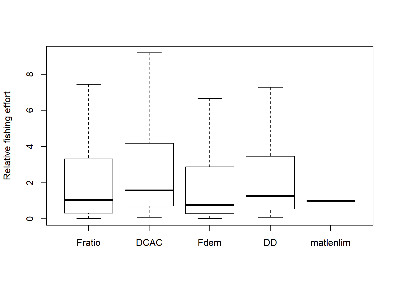
This plot shows that the median fishing effort in the final year ranges from 0.77 to 1.57 for the first four output control methods, and is constant for the input control method (matlenlim).
This is because the output control method adjusts the total allowable catch, which depending on the amount of available stock, also impacts the amount of fishing activity.
The input control methods assume that fishing effort is held at constant levels in the future, although the catchability is able to randomly or systematically vary between years. Furthermore, input control methods can also adjust the amount of fishing effort in each year.