D Assumptions of DLMtool
Like all models, DLMtool is a simplication of reality. In order to approximate real fishery dynamics, DLMtool relies on a number of simplifying assumptions.
Some of these assumptions are common to many fishery science models (e.g., age-structured population dynamics) and are a central to the structure of DLMtool. Other assumptions are a result of the way DLMtool was designed and developed, and may represent limitations of DLMtool for applications to particular situations. It may be possible to deal with some of these assumptions by further development of DLMtool.
D.1 Biology
Short-Lived Species
Due to the problems with approximating fine-scale temporal dynamics with an annual model it is not advised to use the DLMtool for very short lived stocks (i.e., species with a longevity of 5 years or less).
Technically, you could just divide all temporal parameters by a subyear resolution, but the TAC would be set by sub year and the data would also be available at this fine-scale which is highly unlikely in a data-limited setting.
A MSE model with monthly or weekly time-steps for the population dynamics is required for short-lived species, and may be developed in the future.
Density-Dependent Compensation
DLMtool assumes that, with the exception of the stock-recruitment relationship, there is no density-dependent compensation in the population dynamics, and fish growth, maturity, and mortality does not change directly in response to changes in stock size.
von Bertalanffy Growth
Growth model in DLMtool is modelled using the von Bertalanffy growth curve. While this is the most commonly applied model to describe fish growth, it may not be the preferred growth model for some species. The consequences of assuming the von Bertalanffy growth model should be considered when using the DLMtool for species with alternative growth patterns. Since DLMtool V4.4 it is possible to use alternative length-at-age models by using cpars. See the Custom Parameters chapter for more information.
Natural Mortality Rate at Age
By default DLMtool assumes that natural mortality (M) is constant with age and size. Since DLMtool V4.4 size or age-specific M can be specified. See the Size-Specific Natural Mortality chapter for more information.
D.2 MSE Model Assumptions
Retention and Selectivity
The OM has slots for both gear selectivity and retention by size. If the retention slots are not populated, it is assumed that retention = selectivity, that is, all fish that are captured by the gear are retained by the fishers.
Most size-regulation MPs (e.g., matlenlim) change the retention pattern and leave the selectivity pattern unchanged. For example, if a size limited is regulated well above the current size of selection, fish smaller than the size limit are still caught by the gear but are discarded and may suffer some fishing mortality (Stock@Fdisc).
MPs can be designed to modify gear selectivity instead of, or in addition to, the retention-at-size.
Non-Convergence of Management Procedure
In some cases during the MSE Management Procedure may not be able to successfully calculate a management recommendation from the simulated data. For example, a catch-curve may used to estimate \(Z\), and \(F\) is calculated as \(F=Z-M\). Because of process and observation error, it is possible that the estimated \(F\) is negative, in which case the MP may fail to calculate a recommended catch limit.
The Management Procedures have been designed to return NA if they fail to calculate a management recommendation for any reason. In this case, the management recommendations from the previous year are used in the simulation, e.g., \(\text{TAC}_y = \text{TAC}_{y-1}\).
Idealised Observation Models for Catch Composition Data
Currently, DLMtool simulates catch-composition data from the true simulated catch composition data via a multinomial distribution and some effective sample size. This observation model may be unrealistically well-behaved and favour those approaches that use these data. We are considering adding a growth-type-group model to improve the realism of simulated length composition data.
Two-Box Model
DLMtool uses a two-box spatial model and assumes homogeneous fishing, and distribution of the fish stock. That is, growth and other life-history characteristics do not vary across the two spatial areas. Spatial targeting of the fishing fleet is currently being developed in the model.
Ontogenetic Habitat Shifts
Since the operating model simulates two areas, it is possible to prescribe a log-linear model that moves fish from one area to the other as they grow older. This could be used to simulate the ontogenetic shift of groupers from near shore waters to offshore reefs. Currently this feature is in development.
Closed System
DLMtool assumes that the population being modelled is in a closed system. There is no immigration or emigration, and a unit stock is assumed to be represented in the model and impacted by the management decisions. This assumption may be violated where the stock extends across management jurisdictions. Violations of this assumption may impact the interpretation of the MSE results, and these implications should be considered when applying DLMtool.
Although a unit stock is a central assumption of many modeling and assessment approaches, it may be possible to further develop DLMtool to account for stocks that cross management boundaries.
D.3 Management Procedures
Harvest Control Rules Must be Integrated into Data-Limited MPs
In this version of DLMtool, harvest control rules (e.g. the 40-10 rule) must be written into a data-limited MP. There is currently no ability to do a factorial comparison of say 4 harvest controls rules against 3 MPs (the user must describe all 12 combinations). The reason for this is that it would require further subclasses.
For example the 40-10 rule may be appropriate for the output of DBSRA but it would not be appropriate for some of the simple management procedures such as DynF that already incorporate throttling of TAC recommendations according to stock depletion.
D.4 Data and Method Application
Data Assumed to be Representative
The MSE model accounts for observation error in the simulated fishery data. However, the application of management procedures for management advice assumes that the provided fishery data is representative of the fishery and is the best available information on the stock. Processing of fishery data should take place before entering the data into the fishery data tables, and assumptions of the management procedures should be carefully evaluated when applying methods using DLMtool.
D.5 Calculating Reference Points
Biological reference points are used to initialize the simulations (e.g. Depletion) and evaluate the performance of management procedures (e.g., \(B/B_{MSY}\), \(B/B_0\), etc). Although these terms are used frequently, the definition of biological reference points can be ambiguous, and there may be multiple ways of defining or interpreting them. This is especially true when life-history and fishing parameters vary over time.
Here we describe how the biological reference points are defined and calculated in DLMtool.
Depletion and Unfished Reference Points
The Depletion parameter in the Stock Object (Stock@D) is used to initialize the historical simulations. Although the term Depletion is used frequently in fisheries science, it is rarely clearly defined. In most contexts, Depletion is used to mean the biomass today relative to the average unfished biomass. This raises two questions:
- What do we mean by biomass? Is it total biomass (B), vulnerable biomass (VB), or spawning biomass (SB)?
- What do we mean by average unfished biomass? Average over what time-period? Does this refer to the average biomass at some time in history before fishing commenced? Or is the expected biomass today if the stock had not been fished?
Examples can be found for all three definitions of biomass in the first question. We define Depletion with respect to spawning biomass (SB). That is, the values specified in Stock@D refer to the spawning biomass in the last historical year (i.e. ‘today’; \(SB_{y=\text{OM@nyears}}^{\text{unfished}}\)) relative to the average unfished spawning biomass \((SB_0)\).
The answer to the second question is a little more complicated. There are several ways to define \(SB_0\) within the simulation model:
- The unfished spawning biomass at the beginning of the simulations (i.e Year = 1).
- The unfished spawning biomass at the end of the historical simulations (i.e Year =
OM@nyears). - The average unfished spawning biomass over the first several years of the simulations. This could be different to 1 due to inter-annual variability in life-history parameters (e.g,
Stock@Linfsd). - The average unfished spawning biomass over all historical years (or the last several years). This could be different to 3 due to time-varying trends in parameters (e.g., by using
OM@cpars$Linfarray).
In DLMtool the operating model is specified based on the assumed or estimated spawning biomass today relative to the average equilibrium (i.e no process error in recruitment) biomass at the beginning of the fishery; i.e., the change in biomass over the history of the fishery (point 3 above). We use the age of 50% maturity (\(A_{50}\) in the first historical year; calculated internally from Stock@Linf, Stock@Linfsd, Stock@K, Stock@Ksd, Stock@t0, and Stock@L50) as an approximation of generation time, and calculate the average unfished spawning biomass \((SB_0)\) over the first \(A_{50}\) years in the historical simulations. That is:
\[ SB_0 = \frac{\sum_{y=1}^{A_{50}} SB_y^{\text{unfished}}}{A_{50}} \] where \(A_{50}\) is rounded up to the nearest integer and \(SB_y^{\text{unfished}}\) is the equilibrium unfished spawning biomass in year \(y\). The same calculation is used to calculate other unfished reference points (e.g, \(B_0\), \(VB_0\)), as well as the unfished spawning-per-recruit parameters used in the Ricker stock-recruitment relationship.
The unfished reference points and unfished biomass and numbers by year are returned as a list in the MSE and Hist objects; i.e MSE@Misc$Unfished$Refs and `MSE@Misc$Unfished$ByYear respectively.
Note
Note that although Depletion is calculated relative to the average unfished equilibrium spawning biomass, the population in the simulation model is initialized under dynamic conditions, that is, with process error in recruitment to all age classes. This means that, depending on the magnitude of recruitment variability, the initial biomass in Year 1 may be quite different to the equilibrium unfished biomass as calculated above.
D.5.1 Initial Depletion
As noted above, the operating model initializes the population in an unfished dynamic state. Since DLMtool version 5.3 it is possible specify depletion in the first historical year by using OM@cpars$initD. When this feature is used, the population is initialized in a dynamic state with spawning biomass equal to \(\text{initD} * SB_0\); that is, initial spawning biomass in Year 1 is relative to the unfished spawning biomass in Year 1.
Analysts need to be aware that if there are large time-varying trends in life-history parameters, the \(SB_0\) in Year 1, which is no longer the first year that the fishery commenced, may be different to the \(SB_0\) from the (not modeled) period before fishing.
D.5.2 MSY Reference Points
The calculation of maximum sustainable yield (MSY) and related reference points are also impacted by inter-annual variability in life-history and fishing parameters (i.e., selectivity pattern). For example, if there is large inter-annual variability in natural mortality or growth, MSY and \(B_{\text{MSY}}\) may vary significantly between years.
We calculate MSY and related metrics (e.g., \(B_{\text{MSY}}\)) for each time-step in the model based on the life-history and fishing parameters in that year. The MSY reference points are used in both the simulated Data object, and to evaluate the performance of the management procedures.
For the simulated Data object, we calculate MSY reference points following a similar procedure to that described above for \(B_0\). We use \(A_{50}\) as an approximation of generation time, and average the annual MSY values over \(A_{50}\) years around the last historical year. For example, if OM@nyears = 50 and \(A_{50}=5\), \(SB_{\text{MSY}}\) is calculated as:
\[ SB_{\text{MSY}} = \sum_{y=48}^{52}{SB_y^{\text{MSY}}} \] where \(SB_y^{\text{MSY}}\) is the spawning biomass corresponding with maximum sustainable yield in year \(y\). The logic behind this is, if estimates of MSY, \(B_\text{MSY}\), etc are available, they are likely calculated based on current life-history information, which would be estimated from data spanning several age classes.
The MSY reference points in the Data object are not updated in the future projection years. The MSY reference points and MSY values by year are returned in MSE@Misc$MSYRefs.
Note
In DLMtool the MSY metrics are always calculated by year. The slot
MSE@B_BMSYreturns the spawning biomass in the projections divided by \(SB_\text{MSY}\) in each year of the projections. For alternative methods to calculate \(B/B_{\text{MSY}}\), such as relative to the constant \(B_\text{MSY}\) described above, useMSE@SSBorMSE@Band the data stored inMSE@Misc$MSYRefs.
D.5.3 Setting Depletion at a fraction of BMSY
Relative reference points such as \(\frac{B_\text{MSY}}{B_0}\), and \(\frac{SB_\text{MSY}}{SB_0}\) are calculated relative to the unfished biomass described in the previous section. This means that it is relatively straightforward to initialize the simulation model at a fraction of \(B_\text{MSY}\) rather than \(B_0\).
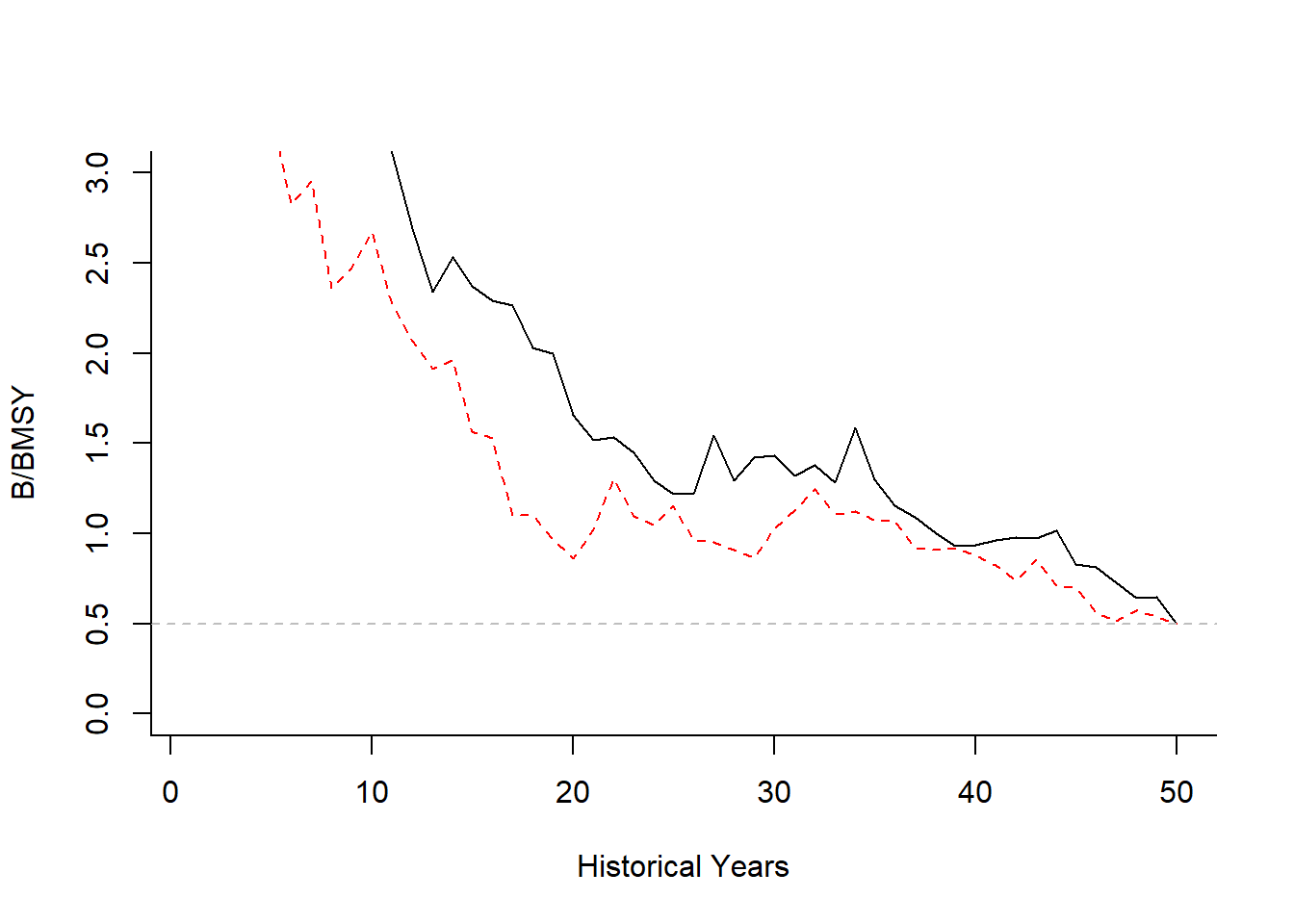
For example, suppose you wish to set the depletion in the final historical year at \(0.5SB_\text{MSY}\):
library(DLMtool)
OM <- testOM; OM@nsim <- 2
OM@cpars$D <- runif(OM@nsim, OM@D[1], OM@D[2]) # need to populate OM@cpars$D so that random samples are the same
Hist <- runMSE(OM, Hist=TRUE, silent=TRUE)
OM@cpars$D <- 0.5 * Hist@Ref$SSBMSY_SSB0 # update Depletion to 0.5 BMSY using cpars
Hist <- runMSE(OM, Hist=TRUE, silent=TRUE)

matplot(t(Hist@TSdata$SSB/Hist@Ref$SSBMSY), type="l", ylim=c(0,3),
        ylab="B/BMSY", xlab="Historical Years", bty="l")
abline(h=0.5, lty=2, col="gray")