Chapter 28 Subsetting the MSE Object

The plotting functions demonstrated above calculate the probabilities and show the trade-offs for all the simulations in the MSE. However, sometimes it is interesting to examine the results of individual Management Procedures or simulations.

Many of the plotting functions have the optional arguments MPs and sims which allow you to specify which particular Management Procedures or simulations to include in the plots.

You can also manually subset the MSE object using the Sub function.

28.1 Subsetting by Performance

For example, we may wish to include only Management Procedures that have greater than 70% probability that the biomass is above \(0.5B_{MSY}\):

We can do this using a combination of the summary function and the Sub function:

stats <- summary(BSharkMSE) # save summary object to `stats`

## Calculating Performance Metrics

##                                       Performance.Metrics                                            
## 1                 Probability of not overfishing (F<FMSY)               Prob. F < FMSY (Years 1 - 50)
## 2                      Spawning Biomass relative to SBMSY         Prob. SB > 0.5 SBMSY (Years 1 - 50)
## 3        Average Annual Variability in Yield (Years 1-50)               Prob. AAVY < 20% (Years 1-50)
## 4 Average Yield relative to Reference Yield (Years 41-50)  Prob. Yield > 0.5 Ref. Yield (Years 41-50)
## 
## 
## Performance Statistics:
##          MP PNOF  P50 AAVY  LTY
## 1    Fratio 0.49 0.60 0.62 0.50
## 2      DCAC 0.57 0.71 0.84 0.62
## 3      Fdem 0.54 0.61 0.70 0.45
## 4        DD 0.50 0.70 0.80 0.71
## 5 matlenlim 0.75 0.88 0.33 0.85

accept <- which(stats$P50 > 0.70) # index of methods that pass the criteria
MPs <- stats[accept,"MP"] # the acceptable MPs

subMSE <- Sub(BSharkMSE, MPs=MPs)

Here we can see that the DCAC, matlenlim methods (2 of the 5) met our specified criteria. We used the Sub function to create a new MSE object that only includes these Management Procedures.

We can than proceed to continue our analysis on the subMSE object, e.g.:

Tplot(subMSE)

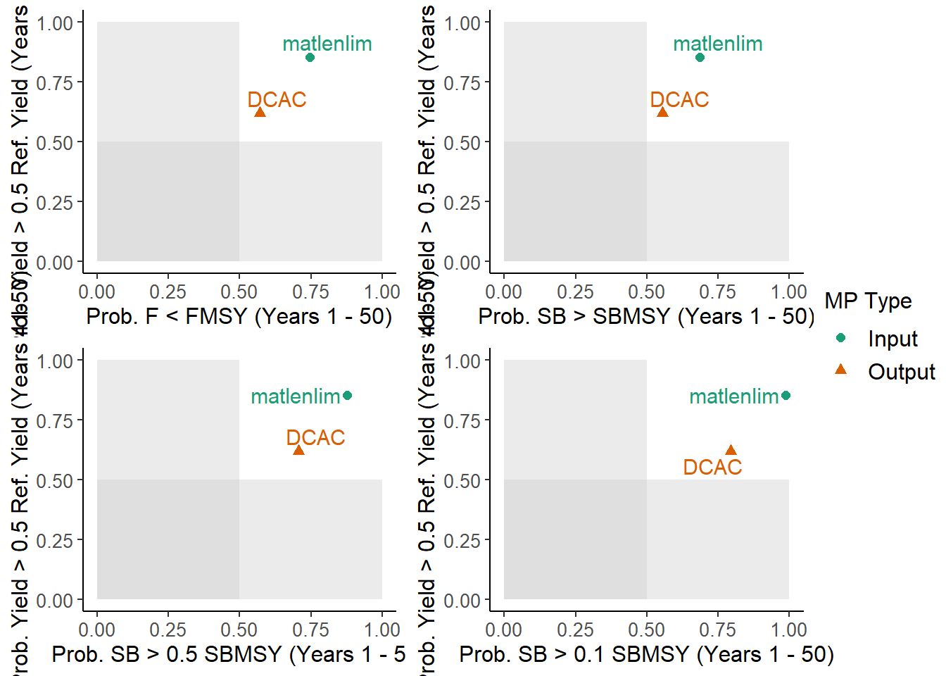
##          MP PNOF  LTY P100  P50  P10 Satisificed
## 1      DCAC 0.57 0.62 0.56 0.71 0.79        TRUE
## 2 matlenlim 0.75 0.85 0.69 0.88 0.99        TRUE

28.2 Subsetting by Operating Model Parameters

We can also subset the MSE object by simulation. For example, we may be interested to look at how the methods perform under different assumptions about the natural mortality rate (M).

In this MSE M ranged from 0.15 to 0.25. Here we identify the simulations where M was below and above the median rate:

below <- BSharkMSE@OM$M < median(BSharkMSE@OM$M)
above <- BSharkMSE@OM$M > median(BSharkMSE@OM$M)

We can then use the Sub function to create two MSE objects, one only including simulations with lower values of M, and the other with simulations where M was above the median value:

belowMSE <- Sub(BSharkMSE, sims=below)
aboveMSE <- Sub(BSharkMSE, sims=above)

You can see that the original MSE object has been split into two objects, each with half of the simulations:

belowMSE@nsim

## [1] 100

aboveMSE@nsim

## [1] 100

We could then continue our analysis on each subset MSE and determine if the natural mortality rate is critical in determining which Management Procedure we would choose as the best option for managing the fishery.