Chapter 29 Custom Performance Metrics

PM methods were introduced in the Performance Metrics Methods chapter. DLMtool includes several built-in PM methods:

avail("PM")

##  [1] "AAVE"  "AAVY"  "LTY"   "P10"   "P100"  "P50"   "PNOF"  "STY"   "Yield" "MeanB" "MeanF"

We saw in Customizing the PM Functions that it is straightforward to modify the years that the performance statistics are calculated over using the Yrs argument, and the reference level using the Ref argument. In this section we describe the PM functions in more detail for advanced users who wish to develop their own PM methods.

We will demonstrate this using the P50 performance metric function as an example.

29.1 Necessity of Complexity

While at first glance the PM functions may appear overly complicated, they are actually quite straightforward. This level of complexity is required because functions of class PM not only return the required performance statistic, but also relevant contextual information.

Imagine we want to develop a function to calculate the probability that \(B > 0.5 B_\text{MSY}\), which we will define as not overfished. We could do something like this:

P_Noverfished <- function(MSEobj) {
  round(apply(MSEobj@B_BMSY >0.5, 2, mean),2)
}

We could increase the flexibility of the function by adding additional arguments to specify the years to calculate the statistic over, but for this demonstration we will keep it simple.

Applying our function to calculate the performance statistic is straightforward:

MSEobj <- runMSE(silent=TRUE) # run an exampe MSE
p_noverfish <- P_Noverfished(MSEobj) # calculate and store our performance statistic
p_noverfish

## [1] 0.80 0.76 0.99 0.87 0.99 0.92

The p_noverfish variable now contains our performance statistic, which we could use to plot or tabulate results. However, the numeric vector returned by P_Noverfished includes no information on what these numbers represent. This makes it difficult to include the results in generic plotting or summary functions. Furthermore, it is easy to imagine that with several similiar performance metric functions, it will be easy to loose track of the meaning of the results unless an elaborate variable naming system is used.

The PM functions have been designed to avoid this problem by returning all information related to the calculation of the performance statistic. Here we calculate the same performance metric using the relevant PM function:

p1 <- P50(MSEobj)

Note that we don’t need to use a descriptive variable name; the p1 variable includes relevant information on the performance metric. Note also that PM function are most often passed directly to plotting or table functions instead of being called and stored directly.

The p1 variable is an object of class PMobj and includes the following slots:

slotNames(p1)

## [1] "Name"    "Caption" "Stat"    "Ref"     "Prob"    "Mean"    "MPs"

The first two slots contain a descriptive name of the performance statistic, and a caption that can be used in plots or summary tables:

p1@Name

## [1] "Spawning Biomass relative to SBMSY"

p1@Caption

## [1] "Prob. SB > 0.5 SBMSY (Years 1 - 50)"

The last two slots contain the results of performance statistic and the names of the MPs:

p1@Mean

## [1] 0.7950000 0.7575000 0.9929167 0.8737500 0.9933333 0.9191667

p1@MPs

## [1] "AvC"       "DCAC"      "FMSYref"   "curE"      "matlenlim" "MRreal"

We will look at the other 3 slots in detail in the next section. The main point here is to demonstrate the using functions of class PM that return objects of class PMobj has the advantage that the function output is completely self-contained and can be used elsewhere without requiring any additional information.

29.2 `PM` Methods in Detail

Let’s go through the P50 function in detail to see how it works:

P50

## function (MSEobj = NULL, Ref = 0.5, Yrs = NULL) 
## {
##     Yrs <- ChkYrs(Yrs, MSEobj)
##     PMobj <- new("PMobj")
##     PMobj@Name <- "Spawning Biomass relative to SBMSY"
##     if (Ref != 1) {
##         PMobj@Caption <- paste0("Prob. SB > ", Ref, " SBMSY (Years ", 
##             Yrs[1], " - ", Yrs[2], ")")
##     }
##     else {
##         PMobj@Caption <- paste0("Prob. SB > SBMSY (Years ", Yrs[1], 
##             " - ", Yrs[2], ")")
##     }
##     PMobj@Ref <- Ref
##     PMobj@Stat <- MSEobj@B_BMSY[, , Yrs[1]:Yrs[2]]
##     PMobj@Prob <- calcProb(PMobj@Stat > PMobj@Ref, MSEobj)
##     PMobj@Mean <- calcMean(PMobj@Prob)
##     PMobj@MPs <- MSEobj@MPs
##     PMobj
## }
## <bytecode: 0x000001d4fb008468>
## <environment: namespace:DLMtool>
## attr(,"class")
## [1] "PM"

Firstly, functions of class PM must have three arguments: MSEobj, Ref, and Yrs:

args(P50)

## function (MSEobj = NULL, Ref = 0.5, Yrs = NULL) 
## NULL

The first argument MSEobj is obvious, an object of class MSE to calculate the performance statistic.
The second argument Ref must have a default value. This is used as reference for the performance statistic, and will be demonstrated shortly.
The third argument Yrs can have a default value of NULL or specify a numeric vector of length 2 with the first and last years to calculate the performance statistic, or a numeric vector of length 1 in which case if it is positive it is the first Yrs and if negative the last Yrs of the projection period.

The first line of a PM function must be Yrs <- ChkYrs(Yrs, MSEobj). This line updates the Yrs variable and makes sure that the specified year indices are valid. For example:

ChkYrs(NULL, MSEobj) # returns all projection years 
ChkYrs(c(1,10), MSEobj) # returns first 10 years 
ChkYrs(c(60,80), MSEobj) # returns message and last 20 years
ChkYrs(5, MSEobj) # first 5 years
ChkYrs(-5, MSEobj) # last 5 years
ChkYrs(c(50,10), MSEobj) # returns an error

When the default value for Yrs is NULL, the Yrs variable is updated to include all projection years:

Yrs <- ChkYrs(NULL, MSEobj)
Yrs

## [1]  1 50

Next we create a new object of class PMobj, and populate the Name slot with a short but descriptive name:

PMobj <- new("PMobj")
PMobj@Name <- "Spawning Biomass relative to SBMSY"

The next line populates the Caption slot with a brief caption including the years over which the performance statistic is calculated. The if statement is not crucial, but avoids the redundant SB > 1 SBMSY in cases where Ref=1.

Next we store the value of the Ref argument in the PMobj@Ref slot so that information is contained in the function output.

PMobj@Ref <- Ref

The Stat slot is an array that stores the variable which we wish to calculate the performance statistic; an output from the runMSE function with dimensions MSE@nsim, MSE@nMPs, and MSE@proyears (or fewer if the argument Yrs != NULL).

In this case we want to calculate a performance statistic related to the biomass relative to BMSY, and so we assign the Stat slot as follows:

PMobj@Stat <- MSEobj@B_BMSY[, , Yrs[1]:Yrs[2]]

Note that we are including all simulations and MPs and indexing the years specified in Yrs.

Next we use the calcProb function to calculate the mean of PMobj@Stat > PMobj@Ref over the years dimension. This results in a matrix with dimensions MSE@nsim, MSE@nMPs:

PMobj@Prob <- calcProb(PMobj@Stat > PMobj@Ref, MSEobj)

Note that in order to calculate a probability the argument to the calcProb function must be a logical array, which is achieved using the Ref slot.

Also note that in this case PMobj@Stat > PMobj@Ref is equivalent to MSEobj@B_BMSY[, , Yrs[1]:Yrs[2]] > 0.5. The PM functions have been designed this way so that in most cases the PMobj@Prob <- calcProb(PMobj@Stat > PMobj@Ref) line is identical in all PM functions and does not need to be modified. The exception to this is if we don’t want to calculate a probability but want the actual mean values of PMobj@Stat, demonstrated in the example below.

In the next line we calculate the mean of PMobj@Prob over simulations using the calcMean function:

PMobj@Mean <- calcMean(PMobj@Prob)

Similiar to the previous line, this line is identical in all PM functions and can be simply copy/pasted from other PM functions without being modified. The Mean slot is a numeric vector of length MSEobj@nMPs with the overall performance statistic, in this case the probability of \(B > 0.5B_\text{MSY}\) across all simulations and years.

Finally, we store the names of the MPs and return the PMobj.

29.3 Creating Example `PMs` and Plot

As an example, we will create another version of DFO_plot using some custom PM functions and a customized version of TradePlot.

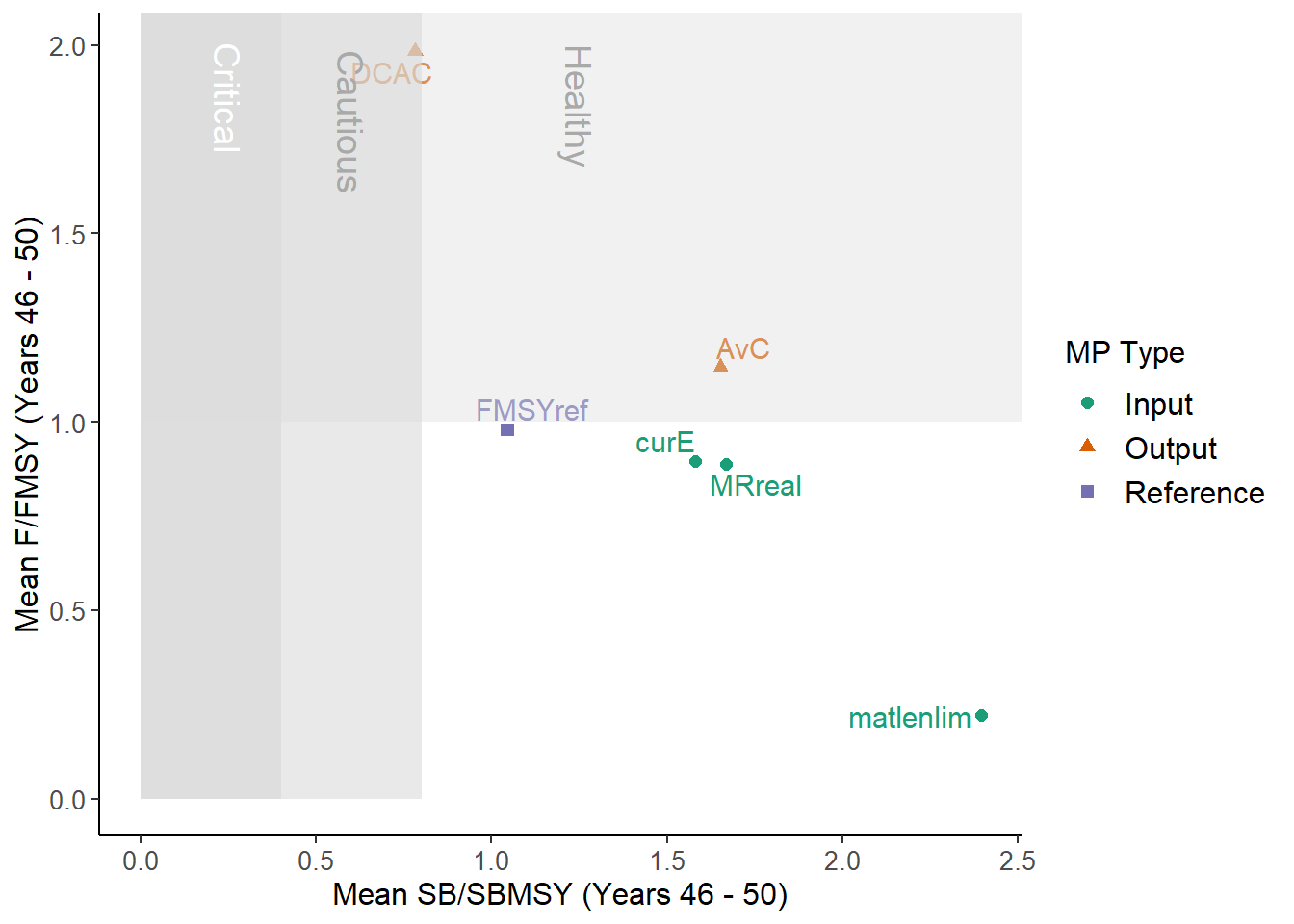
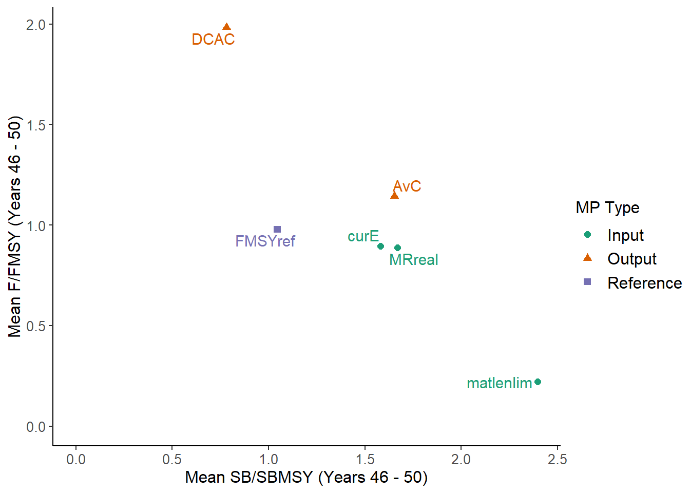
First we create the plot using DFO_plot:

DFO_plot(MSEobj)

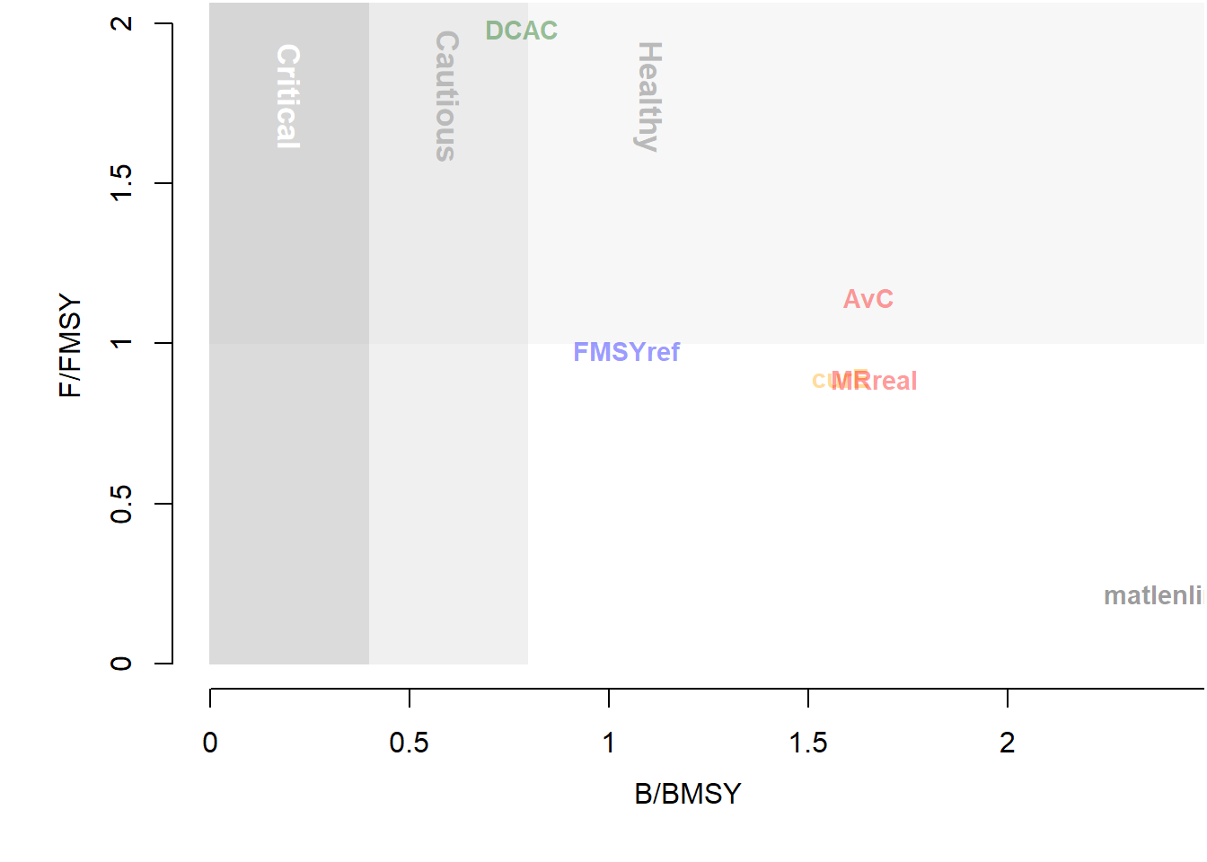
From the help documentation (?DFO_plot) we can see that this function plots mean biomass relative to BMSY and fishing mortality rate relative to FMSY over the final 5 years of the projection.

First we’ll develop a PM function to calculate the mean B/BMSY for the last 5 years of the projection period. Notice that this is very similiar to P50 described above, with the modification of the Caption and the Prob slots, and the Yrs argument. We are calculating a mean here instead of a probability and are not using the Ref argument:

MeanB <- function(MSEobj = NULL, Ref = 1, Yrs = -5) {
    Yrs <- ChkYrs(Yrs, MSEobj)
    PMobj <- new("PMobj")
    PMobj@Name <- "Spawning Biomass relative to SBMSY"
    PMobj@Caption <- paste0("Mean SB/SBMSY (Years ", Yrs[1], " - ", Yrs[2], ")")
    
    PMobj@Ref <- Ref
    PMobj@Stat <- MSEobj@B_BMSY[, , Yrs[1]:Yrs[2]]
    PMobj@Prob <- calcProb(PMobj@Stat, MSEobj)
    PMobj@Mean <- calcMean(PMobj@Prob)
    PMobj@MPs <- MSEobj@MPs
    PMobj
}

We develop a PM function to calculate average F/FMSY in a similar way:

MeanF <- function(MSEobj = NULL, Ref = 1, Yrs = -5) {
    Yrs <- ChkYrs(Yrs, MSEobj)
    PMobj <- new("PMobj")
    PMobj@Name <- "Fishing Mortality relative to FMSY"
    PMobj@Caption <- paste0("Mean F/FMSY (Years ", Yrs[1], " - ", Yrs[2], ")")
    
    PMobj@Ref <- Ref
    PMobj@Stat <- MSEobj@F_FMSY[, , Yrs[1]:Yrs[2]]
    PMobj@Prob <- calcProb(PMobj@Stat, MSEobj)
    PMobj@Mean <- calcMean(PMobj@Prob)
    PMobj@MPs <- MSEobj@MPs
    PMobj
}

Similar to developing custom MPs we need to tell R that these new functions are PM methods:

class(MeanB) <- "PM"
class(MeanF) <- "PM"

Now we can test our performance metric functions:

data.frame(MP=MeanB(MSEobj)@MPs, B_BMSY=MeanB(MSEobj)@Mean, F_FMSY=MeanF(MSEobj)@Mean)

##          MP    B_BMSY    F_FMSY
## 1       AvC 1.6534967 1.1436909
## 2      DCAC 0.7812216 1.9835498
## 3   FMSYref 1.0454687 0.9785792
## 4      curE 1.5807679 0.8960045
## 5 matlenlim 2.3956111 0.2200407
## 6    MRreal 1.6680184 0.8885163

How do these results compare to what is shown in DFO_plot?

We could also use the summary function with our new PM functions, but note that these results are not probabilities:

summary(MSEobj, 'MeanB', 'MeanF')

## Calculating Performance Metrics

##                  Performance.Metrics                               
## 1 Spawning Biomass relative to SBMSY  Mean SB/SBMSY (Years 46 - 50)
## 2 Fishing Mortality relative to FMSY    Mean F/FMSY (Years 46 - 50)
## 
## 
## Performance Statistics:
##          MP MeanB MeanF
## 1       AvC  1.70  1.10
## 2      DCAC  0.78  2.00
## 3   FMSYref  1.00  0.98
## 4      curE  1.60  0.90
## 5 matlenlim  2.40  0.22
## 6    MRreal  1.70  0.89

Finally, we will develop a customized plotting function to reproduce the image produced by DFO_plot.

We can produced something fairly similar quite quickly using the TradePlot function:

TradePlot(MSEobj, 'MeanB', 'MeanF', Lims=c(0,0))

##          MP MeanB MeanF Satisificed
## 1       AvC  1.70  1.10        TRUE
## 2      DCAC  0.78  2.00        TRUE
## 3   FMSYref  1.00  0.98        TRUE
## 4      curE  1.60  0.90        TRUE
## 5 matlenlim  2.40  0.22        TRUE
## 6    MRreal  1.70  0.89        TRUE

Adding the shaded polygons and text requires a little more tweaking and some knowledge of the ggplot2 package. We will wrap up our code in a function:

NewPlot <- function(MSEobj) {
  # create but don't show the plot
  P <- TradePlot(MSEobj, 'MeanB', 'MeanF', Lims=c(0,0), Show=FALSE) 
  P1 <- P$Plots[[1]] # the ggplot objects are returned as a list
  
  # add the shaded regions and the text
  P1 + ggplot2::geom_rect(ggplot2::aes(xmin=c(0,0,0), xmax=c(0.4, 0.8, Inf), 
                                       ymin=c(0,0,1), ymax=rep(Inf,3)),
                          alpha=c(0.8, 0.6, 0.4), fill="grey86") +
    ggplot2::annotate(geom = "text", x = c(0.25, 0.6, 1.25), y = Inf, 
                      label = c("Critical", "Cautious", "Healthy") , 
                      color = c('white', 'darkgray', 'darkgray'), 
                      size=5, angle = 270, hjust=-0.25)

}

NewPlot(MSEobj)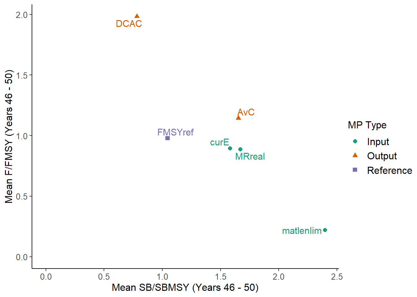

##          MP MeanB MeanF Satisificed
## 1       AvC  1.70  1.10        TRUE
## 2      DCAC  0.78  2.00        TRUE
## 3   FMSYref  1.00  0.98        TRUE
## 4      curE  1.60  0.90        TRUE
## 5 matlenlim  2.40  0.22        TRUE
## 6    MRreal  1.70  0.89        TRUE

Chapter 29 Custom Performance Metrics

29.1 Necessity of Complexity

29.2 PM Methods in Detail

29.3 Creating Example PMs and Plot

29.2 `PM` Methods in Detail

29.3 Creating Example `PMs` and Plot